Results of the ISMRM 2020 joint Reproducible Research & Quantitative MR study groups reproducibility challenge on phantom and human brain T₁ mapping

Purpose: T₁ mapping is a widely used quantitative MRI technique, but its tissue-specific values remain inconsistent across protocols, sites, and vendors. The ISMRM Reproducible Research study group (RRSG) and Quantitative MR study group (qMRSG) jointly launched a T₁ mapping reproducibility challenge. The goal was to investigate whether an independently-implemented image acquisition protocol at multiple centers could reliably measure T₁ using inversion recovery in a standardized phantom and in brains of healthy volunteers.

Methods: The reproducibility of a robust T₁ mapping protocol and fitting algorithm from a well-known Magnetic Resonance in Medicine publication (Barral et al. 2010) were evaluated. Participants in the challenge were invited to acquire T₁ mapping data on a standard ISMRM/NIST phantom and/or in healthy human brains. Data submission, pipeline development, and analysis were performed using open-source platforms for increased reproducibility and transparency. For participants acquiring data at multiple sites, inter-submission and intra-submission comparisons were conducted by selecting one dataset per submission.

Results: Eighteen submissions were accepted using data collected from MRIs from three manufacturers (Siemens, GE, Philips) and at 3T (except one submission, at 0.35T), resulting in a total of 38 datasets acquired in phantoms and 56 datasets in healthy human subjects. Inter-submission mean coefficient of variation (CoV) was 6.1% for phantom measurements, nearly twice as high as the evaluated intra-submission CoV (2.9%). A similar trend was observed in the human data (inter-/intra- submission CoV was 6.0/2.9 % in the genu and 16/6.9 % in the cortical gray matter).

Conclusion: The imaging protocol and fitting algorithm from Barral et al. (2010) resulted in good reproducibility of both phantom and human brain T₁ measurements. Differences in implementations between submissions resulted in higher variance in reported values relative to intra-submission variability. This challenge generated a large open database of inversion recovery T₁ mapping acquisitions across several sites and MRI vendors accessible at osf.io/ywc9g/. To allow for the wider community to access and engage with this dataset, we developed an interactive dashboard that is available at https://rrsg2020.dashboards.neurolibre.org.

Dashboard: Challenge Submissions

+++

1| introduction¶

Significant challenges exist in the reproducibility of quantitative MRI (qMRI) Keenan et al., 2019. Despite its promise of improving the specificity and reproducibility of MRI acquisitions, few qMRI techniques have been integrated into clinical practice. Even the most fundamental MR parameters cannot be measured with sufficient reproducibility and precision across clinical scanners to pass the second of six stages of technical assessment for clinical biomarkers Fryback & Thornbury, 1991Schweitzer, 2016Seiberlich et al., 2020. Half a century has passed since the first quantitative T₁ (spin-lattice relaxation time) measurements were first reported as a potential biomarker for tumors Damadian, 1971, followed shortly thereafter by the first in vivo quantitative T₁ maps Pykett & Mansfield, 1978 of tumors, but there is still disagreement in reported values for this fundamental parameter across different sites, vendors, and implementations Stikov et al., 2015.

Among fundamental MRI parameters, T₁ holds significant importance Boudreau et al., 2020. It represents the time it takes for the longitudinal magnetization to recover after being disturbed by an RF pulse. The T₁ value varies based on molecular mobility and magnetic field strength Bottomley et al., 1984Dieringer et al., 2014Wansapura et al., 1999, making it a valuable parameter for distinguishing different tissue types. Accurate knowledge of T₁ values is essential for optimizing clinical MRI pulse sequences for contrast and time efficiency Ernst & Anderson, 1966Redpath & Smith, 1994Tofts, 1997 and as a calibration parameter for other quantitative MRI techniques Sled & Pike, 2001Yuan et al., 2012. Among the number of techniques to measure T₁, inversion recovery (IR) Drain, 1949Hahn, 1949 is widely held as the gold standard technique, as it is robust against other effects (e.g. B₁ inhomogeneity) and potential errors in measurements (e.g. insufficient spoiling) Stikov et al., 2015. However, because the technique requires a long repetition time (TR > T₁), it is very slow and impractical for whole-organ measurements, limiting its clinical use. In practice, it is mostly used as a reference to validate other T₁ mapping techniques, such as variable flip angle imaging (VFA) Cheng & Wright, 2006Deoni et al., 2003Fram et al., 1987, Look-Locker Look & Locker, 1970Messroghli et al., 2004Piechnik et al., 2010, and MP2RAGE Marques et al., 2010Marques & Gruetter, 2013.

Efforts have been made to develop quantitative MRI phantoms to assist in standardizing T₁ mapping methods Keenan et al., 2018. A quantitative MRI standard system phantom was created in a joint project between the International Society for Magnetic Resonance in Medicine (ISMRM) and the National Institute of Standards and Technology (NIST) Stupic et al., 2021, and has since been commercialized (Premium System Phantom, CaliberMRI, Boulder, Colorado). The spherical phantom has a 57-element fiducial array containing spheres with doped liquids that model a wide range of T₁, T₂, and PD values. The reference values of each sphere were measured using NMR at 3T Stupic et al., 2021. The standardized concentration for relaxometry values established as references by NIST are also used by another company for their relaxometry MRI phantoms (Gold Standard Phantoms Ltd., Rochester, England). The cardiac TIMES phantom Captur et al., 2016 is another commercially available system phantom focusing on T₁ and T₂ values in blood and heart muscles, pre- and post-contrast. The ISMRM/NIST phantom has been used in several large multicenter studies already, for example in Bane et al., 2018 where they compared measurements at eight sites on a single ISMRM/NIST phantom using the inversion recovery and VFA T₁ mapping protocols recommended by NIST, as well as some site-specific imaging protocols used for dynamic contrast enhanced (DCE) imaging. Bane et al. (2018) concluded that the acquisition protocol, field strength, and T₁ value of the sample impacted the level of accuracy, repeatability, and interplatform reproducibility that was observed. In another study led by NIST researchers Keenan et al., 2021, T₁ measurements were done at two clinical field strengths (1.5T and 3.0 T) and 27 MRI systems (three vendors) using the recommended NIST protocols. That study, which only investigated phantoms, found no significant relationship between T₁ discrepancies of the measurements and the MRI vendors used.

The 2020 ISMRM reproducibility challenge ^[1] posed the following question:

Will an imaging protocol independently-implemented at multiple centers reliably measure what is considered one of the fundamental MR parameters (T₁) using the most robust technique (inversion recovery) in a standardized phantom (ISMRM/NIST system phantom) and in the healthy human brain?

More broadly, this challenge aimed at assessing the reproducibility of a qMRI method presented in a seminal paper, Barral et al., 2010, by evaluating the variability in measurements observed by different research groups that implemented this imaging protocol. As the focus of this challenge was on reproducibility, the challenge design emphasized the use of reproducible research practices, such as sharing code, pipelines, data, and scripts to reproduce figures.

2| methods¶

2.1| Phantom and human data¶

The phantom portion of the challenge was launched for those with access to the ISMRM/NIST system phantom Stupic et al., 2021 (Premium System Phantom, CaliberMRI, Boulder, Colorado). Two versions of the phantom have been produced with slightly different T₁/T₂/PD values in the liquid spheres, and both versions were used in this study. Phantoms with serial numbers 0042 or less are referred to as “Version 1”, and those with 0043 or greater are “Version 2”. The phantom has three plates containing sets of 14 spheres for ranges of proton density (PD), T₁ (NiCl2), and T₂ (MnCl2) values. Reference T₁ values at 20 °C and 3T for the T₁ plate are listed in Table 1 for both versions of the phantom. Researchers that participated in the challenge were instructed to record the temperature before and after scanning the phantom using the phantom’s internal thermometer. Instructions for positioning and setting up the phantom were devised by NIST after they had designed the phantom (prior to the challenge), and were provided to participants through the NIST website ^[2]. In brief, instructions included details about how to orient the phantom consistently at different sites, and how long the phantom should be in the scanner room prior to scanning so that a thermal equilibrium was achieved prior to scanning.

Participants were also instructed to collect T₁ maps in the brains of healthy human participants, if possible. To ensure consistency across datasets, single-slice positioning parallel to the anterior commissure - posterior commissure (AC-PC) line was recommended. Before the scanning process, the participants granted their consent ^[4] to share their de-identified data openly with the challenge organizers and on the website Open Science Framework (OSF.io). As the submitted single-slice inversion recovery images would be along the AC-PC line, they are unlikely to contain sufficient information for facial identification, and therefore participants were not instructed to de-face their data. The researchers who submitted human data for the challenge provided written confirmation to the organizers that their data was acquired in accordance with their institutional ethics committee (or equivalent regulatory body) and that the subjects had consented to sharing their data as described in the challenge.

2.2| Protocol¶

Participants were instructed to acquire the T₁ mapping data using the spin-echo inversion recovery protocol for T₁ mapping as reported in Barral et al., 2010, and detailed in Table 2. This protocol uses four inversion times optimized for human brain T1 values and uses a relatively short TR (2550 ms). It is important to note that this acquisition protocol is not suitable for T₁ fitting models that assume TR > 5T₁. Instead, more general models of inversion recovery, such as the Barral et al. (2010) fitting model described in Section 2.4.1, can be used to fit this data.

Researchers who participated in the challenge were advised to adhere to this protocol as closely as possible, and to report any differences in protocol parameters due to technical limitations of their scanners and/or software. It was recommended that participants submit complex data (magnitude and phase, or real and imaginary), but magnitude-only data was also accepted if complex data could not be conveniently exported.

2.3| Data Submissions¶

Data submissions for the challenge were managed through a dedicated repository on GitHub, accessible at https://github.com/rrsg2020/data_submission. This allowed transparent and open review of the submissions, as well as standardization of the process. All datasets were converted to the NIfTI file format, and images from different TIs needed to be concatenated into the fourth (or “time”) dimension. Magnitude-only datasets required one NIfTI file, while complex datasets required two files (magnitude and phase, or real and imaginary). Additionally, a YAML (*.yaml) configuration file containing submission, dataset, and acquisition details (such as data type, submitter name and email, site details, phantom or volunteer details, and imaging protocol details) was required for each submitted dataset to ensure that the information was standardized and easily found. Each submission was reviewed to confirm that guidelines were followed, and then datasets and configuration files were uploaded to OSF.io (osf.io/ywc9g). A Jupyter Notebook Beg et al., 2021Kluyver et al., 2016 pipeline was used to generate T₁ maps using qMRLab Cabana et al., 2015Karakuzu et al., 2020 and quality-check the datasets prior to accepting the submissions; in particular, we assured that the NiCL₂ array was imaged, that the DICOM images were correctly converted to NIfTI, the each images for each acquired TI were not renormalized (in particular, Philips platforms have different image export options that changes how the images are scaled, and a reconversion was necessary to ensure proper scaling for quantitative imaging in some cases – see the submissions GitHub issue #5 for one example ^[5]) for the purposes of quality assurance. Links to the Jupyter Notebook for reproducing the T₁ map were shared using the MyBinder platform in each respective submission GitHub issue, ensuring that computational environments (eg, software dependencies and packages) could be reproduced to re-run the pipeline in a web browser.

2.4| Data Processing¶

2.4.1| Fitting Model and Pipeline¶

A reduced-dimension non-linear least squares (RD-NLS) approach was used to fit the complex general inversion recovery signal equation:

where a and b are complex constants. This approach, introduced in , models the general T₁ signal equation without the long-TR approximation. The a and b constants inherently factor TR in them, as well as other imaging parameters (eg, excitation and refocusing flip angles, TE, etc). Barral et al. (2010) shared the implementation of the fitting algorithm used in their paper ^[6]. Magnitude-only data were fitted to a modified-version of [1] (Eq. 15 of Barral et al. (2010)) with signal-polarity restoration. To facilitate its use in our pipelines, a wrapper was implemented around this code available in the open-source software qMRLab Cabana et al., 2015Karakuzu et al., 2020, which provides a commandline interface (CLI) to call the fitting in MATLAB/Octave scripts.

A Jupyter Notebook data processing pipeline was written using MATLAB/Octave. This pipeline automatically downloads all the datasets from the data-hosting platform osf.io (osf.io/ywc9g), loads each dataset configuration file, fits the T₁ data voxel-wise, and exports the resulting T₁ map to the NIfTI and PNG formats. This pipeline is available in a GitHub repository (https://github.com/rrsg2020/t1_fitting_pipeline, filename: RRSG_T1_fitting.ipynb). Once all submissions were collected and the pipeline was executed, the T₁ maps were uploaded to OSF (osf.io/ywc9g).

2.4.2| Image Labeling & Registration¶

A schematic of the phantom is shown in Figure 1-a. The T₁ plate (NiCl₂ array) of the phantom has 14 spheres that were labeled as the regions-of-interest (ROI) using a numerical mask template created in MATLAB, provided by NIST researchers (Figure 1-b). To avoid potential edge effects in the T₁ maps, the ROI labels were reduced to 60% of the expected sphere diameter. A registration pipeline in Python using the Advanced Normalization Tools (ANTs) Avants et al. (2009) was developed and shared in the analysis repository of our GitHub organization (https://github.com/rrsg2020/analysis, filename: register_t1maps_nist.py, commit ID: 8d38644). Briefly, a label-based registration was first applied to obtain a coarse alignment, followed by an affine registration (gradientStep: 0.1, metric: cross correlation, number of steps: 3, iterations: 100/100/100, smoothness: 0/0/0, sub-sampling: 4/2/1) and a BSplineSyN registration (gradientStep:0.5, meshSizeAtBaseLevel:3, number of steps: 3, iterations: 50/50/10, smoothness: 0/0/0, sub-sampling: 4/2/1). The ROI labels template was nonlinearly registered to each T₁ map uploaded to OSF.

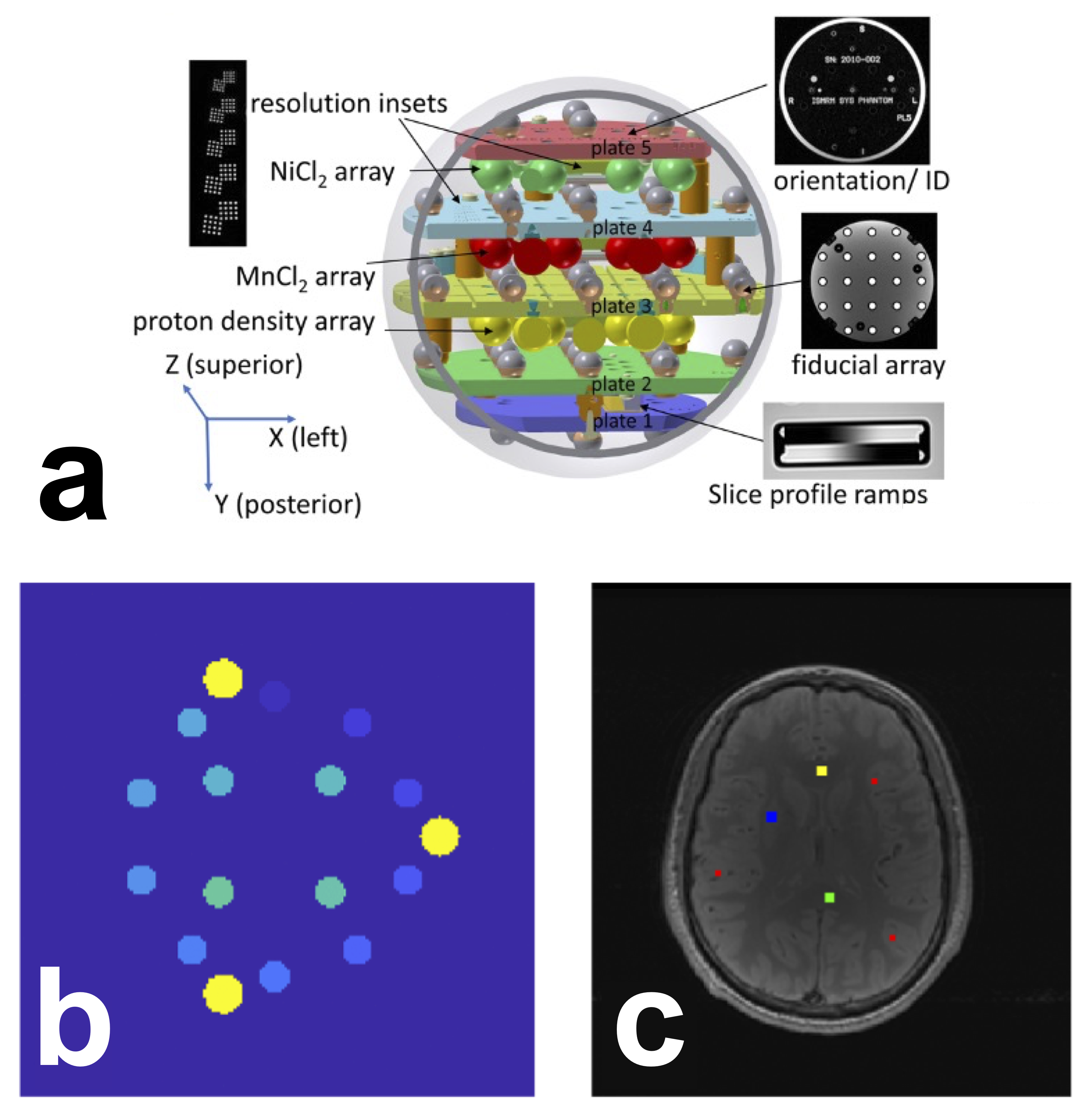
Figure 1 Schematic of the system phantom (a) used in this challenge. Reproduced and cropped from Stupic et al. 2021 (Stupic et al. 2021) (Creative Commons CC BY license). ROI selection for the ISMRM/NIST phantom (b) and the human brain (c). b) The 14 phantom ROIs (shades of blue/green) were automatically generated using a script provided by NIST. In yellow are the three reference pins in the phantom, i.e. these are not ROIs or spheres. c) Human brain ROIs were manually segmented in four regions: the genu (yellow, 5⨯5 voxels), splenium (green, 5⨯5 voxels), deep gray matter (blue, 5⨯5 voxels), and cortical gray matter (red, three sets of 3⨯3 voxels). Note: due to differences in slice positioning from the single-slice datasets provided by certain sites, for some datasets it was not possible to manually segment an ROI in the genu or deep gray matter. In the case of the missing genu, left or right frontal white matter (WM) was selected; for deep gray matter (GM), it was omitted entirely for those cases.

Manual ROIs were segmented by a single researcher (M.B., 11+ years of neuroimaging experience) using FSLeyes McCarthy, 2022 in four regions for the human datasets Figure 1-c): located in the genu, splenium, deep gray matter, and cortical gray matter. Automatic segmentation was not used because the data were single-slice and there was inconsistent slice positioning between datasets.

2.4.3| Analysis and Statistics¶

Analysis code and scripts were developed and shared in a version-tracked public GitHub repository ^[7]. T₁ fitting and main data analysis was performed for all datasets by one of the challenge organizers (M.B.). Python-based Jupyter Notebooks were used for both the quality assurance and main analysis workflows. The computational environment requirements were containerized in Docker Boettiger, 2015Merkel, 2014, allowing for an executable environment that can reproduce the analysis in a web browser through MyBinder ^[8] Project Jupyter et al., 2018. Python scripts handled reference data, database handling, ROI masking, and general analysis tools, while configuration files managed the dataset information which were downloaded and pooled using a script (make_pooled_datasets.py). The databases were created using a reproducible Jupyter Notebook and subsequently saved in the repository.

For the ISMRM/NIST phantom data, mean T₁ values for each ROI were compared with temperature-corrected reference values and visualized in three different types of plots (linear axes, log-log axes, and error relative to the reference value). This comparison was repeated for individual measurements at each site and for all measurements grouped together. Temperature correction was carried out via nonlinear interpolation ^[9] of the set of reference NIST T₁ values between 16 °C and 26 °C (2 °C intervals), listed in the phantom technical specifications. For the human datasets, a notebook was created to plot the mean and standard deviations for each tissue ROI from all submissions from all sites. All quality assurance and analysis plot images were saved to the repository for ease-of-access and a timestamped version-controlled record of the state of the analysis figures. The database files of ROI values and acquisition details for all submissions were also saved to the repository.

An interactive dashboard ^[10] was developed in Dash by Plotly (Plotly Technologies Inc. 2015) and hosted by NeuroLibre Karakuzu et al., 2022 to enable real-time exploration of the data, analysis, and statistics of the challenge results. The dashboard reports descriptive statistics for a variety of alternative looks at phantom and brain data, as well as some statistical comparisons (e.g., the hierarchical shift function ^[11]). The data was collected from the pre-prepared databases of masked ROI values and incorporated other database information, such as phantom version, temperature, MRI system, and reference values. The interactive dashboard displays these results for all measurements at all sites.

3| results¶

3.1| Dashboard¶

To disseminate the challenge results, a web-based dashboard was developed (Figure 2, https://rrsg2020.dashboards.neurolibre.org). The landing page (Figure 2-a) showcases the relationship between the phantom and brain datasets acquired at different sites/vendors. Navigating to the phantom section leads to the information about the submitted datasets, such as the mean/std/median/CoV for each sphere, % difference from the reference values, number of scans, and temperature (Figure 2-b, left). Other options allow users to limit the results by specific versions of the phantom or the MRI manufacturer. Selecting either “By Sphere” (Figure 2-b, right) or “By Site” tabs will display whisker plots for the selected options, enabling further exploration of the datasets.

Returning to the home page and selecting the brain section allows exploration of information on the brain datasets (Figure 2-c, left), such as mean T₁ and STD for different ROI regions, as well as selection of specific MRI manufacturers. Choosing the “By Regions” tab provides whisker plots of the datasets for the selected ROI (Figure 2-c, right), similar to the plots for the phantom.

Figure 2 Dashboard. a) welcome page listing all the sites, the types of subject, and scanner, and the relationship between the three. Row b) shows two of the phantom dashboard tabs, and row c) shows two of the human data dashboard tabs Link: https://rrsg2020.dashboards.neurolibre.org

3.2| Submissions¶

Eighteen submissions were included in the analysis, which resulted in 38 T₁ maps of the NIST/system phantom, and 56 brain T₁ maps. Figure 3 illustrates all the submissions that acquired phantom data (Figure 3-a) and human data (Figure 3-b), the number of scanners used for each submission, and the number of T₁ mapping datasets. It should be noted that these numbers include a subset of measurements where both complex and magnitude-only data from the same acquisition were used to fit T₁ maps, thus the total number of unique acquisitions is lower than the numbers reported above (27 for phantom data and 44 for human data). The datasets were collected on three MRI manufacturers (Siemens, GE, Philips) and were acquired at 3T ^[12], except for one dataset acquired at 0.35T (the ViewRay MRidian MR-linac) . To showcase the heterogeneity of the actual T₁ map data from the independently-implemented submissions, Figure 4 displays six T₁ maps of the phantoms submitted to the challenge.

Of these datasets, several submissions went beyond the minimum acquisition and acquired additional datasets using the ISMRM/NIST phantom, such as a traveling phantom (7 scanners/sites), scan-rescan, same-day rescans on two MRIs, short TR vs long TR, and 4 point TI vs 14 point TI. For humans, one site acquired 13 subjects on two scanners (different manufacturers), one site acquired 6 subjects, and one site acquired a subject using two different head coils (20 channels vs. 64 channels).

3.3| Phantom¶

An overview of the T₁ results for the submitted ISMRM/NIST phantom datasets is displayed in Figure 5. The same data is presented in each column with different axes types (linear, log, and error) to better visualize the results. Figure 5-a shows good agreement (slope = 0.98, intercept = -14 ms) for this dataset in comparison to the reference T₁ values. However, this trend did not persist for low T₁ values (T₁ smaller than 100-200 ms), as seen in the log-log plot (Figure 5-b), which was expected because the imaging protocol is optimized for human water-based T₁ values (T₁ higher than 500 ms). Errors exceeding 10% are observed for T₁ values of phantom spheres below this threshold (Figure 5-c). These trends are observed for the entire-dataset plots as well (Figure 5 d-f). More variability is seen in Figure 5-d around the identity diagonal at very high T₁ (T₁ ~ 2000 ms) than towards the WM-GM values (T₁ ~ 600-1400 ms), which is less apparent in the log-log plot (Figure 5-e). In addition to the low T₁ values exceeding the 10% error threshold (Figure 5-f), a few measurements with outlier values exceeding 10% error (~3-4) were observed in the human water-based tissue range (~500-2000 ms).

Inter-submission coefficients of variation (CoV) were calculated by selecting ad hoc one single T₁ map submitted per challenge participant ^[13] and calculating the CoV of the T₁ means per sphere. The average inter-submission CoV across the first five spheres representing the expected T₁ value range in the human brain (~ 500 to ~ 2000 ms) was 6.1 % (sphere 1 = 4.7 %, sphere 2 = 3.1 %, sphere 3 = 6.3 %, sphere 4 = 12.8 %, sphere 5 = 7.3 %). Two sites were clear outliers that had particular issues for sphere 4, likely because the signal null for this particular T₁ value (~600 ms) is near the second TI and these outliers incorrectly flip the signal at the near-null TI during magnitude-only data fitting ^[14]; by removing these outliers, the mean inter-submission CoV reduces to 4.1 % (sphere 1 = 5.4 %, sphere 2 = 3. 5%, sphere 3 = 2.5 %, sphere 4 = 4.2 %, sphere 5 = 4.9 %). One participant measured T₁ maps with one phantom using one implemented protocol (identical imaging parameters) at 7 different sites on systems from a single manufacturer at 3T, and so a mean intra-submission CoV across the first five spheres for this case was calculated to be 2.9 % (sphere 1 = 4.9 %, sphere 2 = 3.5 %, sphere 3 = 2.6 %, sphere 4 = 2.0 %, sphere 5 = 1.6 %).

Figure 6 compares the mean T₁ values measured using complex and magnitude-only data for the 11 datasets where authors provided both in their submissions. Note that these datasets are from the same acquisition, not two unique acquisitions. The scatter plot shows that for the range of T₁ values expected in the brain (T₁ > 500 ms), there is almost no difference in fitted T₁ values between the two types of data (the highest outlier indicates ~9 ms difference). However, for T₁ values less than ~250 ms large errors ^[15] were present, likely due to the data acquisition imaging protocol (specifically, TI range) being sub-optimal for this range of T₁ values.

The direction of the measurement error in the phantom is influenced by both the measurement site and the reference value, as indicated by the individual shift functions (Figure 7). For example, at sphere 1 (~2000 ms), nearly half of the measurements (20 shown in total) are positioned on each side of the zero-crossing. On the other hand, for sphere 3 (~1s), nearly all the measurements show underestimation as shift functions are located below the zero-crossing. Bootstrapped differences capture these trends, indicating a dominant overestimation at sphere 1 (median difference of +17 ms) and underestimation at sphere 3 (median difference of -39 ms). High-density intervals associated with these median differences do not indicate a common pattern for the former (intervals cross zero), whereas they reveal a notable underestimation trend at sphere 3 (intervals do not include zero). A similar common pattern is also observed for sphere 2 (median overestimation of 35 ms). In addition, the shape of individual shift functions conveys information about how voxel-wise distributions differ. For example, some outliers are observed with these graphs (two by looking at sphere 4). After looking at the T₁ maps, these were not due to mispositioning of ROIs but due to the acquired T₁ mapping data not fitting well for all spheres relative to the reference values. This produced the worse agreement for sphere 4 (these outliers for sphere 4 can also be seen in Figure 5-f). Lastly, the spread of shift functions around the zero-crossing does not indicate vendor-specific clustering for the selected measurements and reference values.

3.4| Human¶

Figure 8 summarizes the results from human datasets submitted to this challenge, showing mean and standard deviation T₁ values from the WM (genu) and GM (cerebral cortex) ROIs. The top plot collapses all datasets for each site, while the bottom plot shows each dataset separately. Mean WM T₁ values across all submissions was 828 ± 38 ms in the genu and 854 ± 50 ms in the splenium, and mean GM T₁ values were 1548 ± 156 ms in the cortex and 1188 ± 133 ms in the deep GM, with less variations overall in WM compared to GM, possibly due to better ROI placement and less partial voluming in WM. Inter-submission coefficients of variation (CoV) for independently-implemented imaging protocols were calculated using one T₁ map measurement per submission that most closely matched the proposed protocol, and were 6.0% for genu, 11% for splenium, 16% for cortical GM and 22% for deep GM. One site (site 9) measured multiple subjects on three scanners using two different vendors, and so intra-submission CoVs for these centrally-implemented protocols were calculated over acquired T₁ maps from this site, and were 2.9% for genu, 3.5% for splenium, 6.9 % for cortical GM and 7.8% for deep GM. This particular acquisition had an ideal slice positioning, cutting through the AC-PC line and the genu for proper ROI placement, particularly for the corpus callosum and deep GM (Supplementary Figure 1 - top left).

3.5| discussion¶

3.6| Achievements of the challenge¶

The challenge focused on exploring the reproducibility of the gold standard inversion recovery T1 mapping method reported in a seminal paper Barral et al., 2010. Eighteen submissions independently implemented the inversion recovery T1 mapping acquisition protocol as outlined in Barral et al. (2010)(which is optimized for the T1 values observed in brain tissue), and reported T1 mapping data in a standard quantitative MRI phantom and/or human brains at 27 MRI sites, using systems from three different vendors (GE, Philips, Siemens). The collaborative effort produced an open-source database of 94 T1 mapping datasets, including 38 ISMRM/NIST phantom and 56 human brain datasets. A standardized T1 processing pipeline was developed for different dataset types, including magnitude-only and complex data. Additionally, Jupyter notebooks that can be executed in containerized environments were developed for quality assurance, visualization, and analyses. An interactive web-based dashboard was also developed to allow for easy exploration of the challenge results in a web-browser.

To evaluate the accuracy of the resulting T₁ values, the challenge used the standard ISMRM/NIST phantom with fiducial spheres having T₁ values in the range of human brain tissue, from 500 to 2000 ms (see Figure 5). As anticipated for this protocol, there was a decrease in the accuracy in measurements for spheres with T₁ below 300 ms. Overall, the majority of the independently implemented imaging protocols from various sites are consistent with the temperature-corrected reference values, with only a few exceptions. Using the NIST phantom, we report that sites that independently implemented the imaging protocol resulted in an inter-submission mean CoV (6.1 %) that was twice as high as the intra-submission mean CoV measured at seven sites (2.9 %). A similar trend was observed in vivo. Inter-submission CoV for WM (genu) was 6.0 % and for GM (cortex) was 16.5 % vs the intra-submission CoV that was 2.9 % and 6.9%, with generally higher CoVs relative to the phantom measurements likely due to biological variability Piechnik et al., 2013Stanisz et al., 2005.

3.7| Comparison with other studies¶

The work done during this challenge involved a multi-center quantitative T₁ mapping study using the NIST phantom across various sites. This work overlaps with two recent studies Bane et al., 2018Keenan et al., 2021. Bane et al. (2018) focused on the reproducibility of two standard quantitative T₁ techniques (inversion recovery and variable flip angle) and a wide variety of site-specific T₁ mapping protocols for DCE, mostly VFA protocols with fewer flip angles, which were implemented at eight imaging centers covering the same 3 MRI vendors featured in this challenge (GE/Philips/Siemens). The inter-platform coefficient of variation for the standard inversion recovery T₁ protocol was 5.46% at 3 T in Bane et al., 2018, which was substantially lower than what they observed for their standard VFA protocol (22.87%). However, Bane et al.’s work differed from the challenge in several ways. First, the standard imaging protocol for inversion recovery used by Bane et al. (2018) had more inversion times (14 compared to the challenge’s 4) to cover the entire range of T₁ values of the phantom. Secondly, Bane et al. (2018) used a single traveling phantom for all sites, whereas the challenge used a total of 8 different phantoms (some were shared amongst people who participated independently). Thirdly, Bane et al. (2018) averaged the signals within each ROI of each sphere prior to fitting for the T₁ values, whereas the challenge pipeline fits the T₁ values on a per-voxel basis and only subsequently calculates the mean/median/std. They also only acquired magnitude data, in contrast to the challenge where participants were encouraged to submit both complex and magnitude-only data. Lastly, in Bane et al. (2018), the implementations of the common inversion recovery protocols were fully standardized (full protocol) across all the platforms (except for two cases where one manufacturer couldn’t achieve the lowest TI) and imposed and coordinated by the principal researchers. In contrast, the challenge sought to explore the variations that would occur for a less-restricted protocol (Table 2) that is independently-implemented at multiple centers, which more closely emulates the quantitative MR research flow (publication of a technique and protocol → independently implement the pulse sequence and/or protocol → use the new implementation independently in a study → publish). Of note, in the challenge, one participating group coordinated a large multicenter dataset that mirrors the study by Bane et al. (2018) by imaging a single phantom across 7 different imaging sites, albeit doing so on a single manufacturer. Using this subset, the mean cross-site CoV was 2.9 % (range: 1.6 - 4.9 %) for the first five spheres, which is in agreement with the range of observations for all spheres by Bane et al. (Bane et al. 2018) at 3T using their full inversion recovery protocol (CoV = 5.46 %; range: 0.99 - 14.6 %).

Another study by Bane et al. (2018)Keenan et al. (2021) also investigated the accuracy of T₁ mapping techniques using a single ISMRM/NIST system phantom at multiple sites and on multiple platforms. Like Bane et al. (2018) they used an inversion recovery imaging protocol optimized for the full range of T₁ values represented in the ISMRM/NIST phantom, which consisted of 9 to 10 inversion times and a TR of 4500 ms (TR ~ 5T₁ of WM at 3T). They reported no consistent pattern of differences in measured inversion recovery T₁ values across MRI vendors for the two T₁ mapping techniques they used (inversion recovery and VFA). They observed relative errors between their T₁ measurements and the reference values of the phantom to be below 10% for all T₁ values and the larger errors were observed at the lowest and highest T₁ values of the phantom.

3.8| Lessons Learned and Future Directions¶

There are some important things to note about this challenge. Firstly, the submissions for this challenge were due in March 2020, which was impacted by the COVID-19 pandemic lockdowns, thereby reducing repeated experiments due to access limitations. Nevertheless, a substantial number of participants submitted their datasets. Some groups intended on acquiring more data, and others intended on re-scanning volunteers, but could no longer do so due to local pandemic restrictions.

This reproducibility challenge aimed to compare differences between independently-implemented protocols. Crowning a winner was not an aim of this challenge, due to concerns that participants would have changed their protocols to get closer to the reference T₁ values, leading to a broader difference in protocol implementations across MRI sites. Instead, we focused on building consensus by creating an open data repository, sharing reproducible workflows, and presenting the results through interactive visualizations. Future work warrants the study of inter-site differences in a vendor-neutral workflow Karakuzu et al., 2022 by adhering to the latest Brain Imaging Data Structure (BIDS) community data standard on qMRI Karakuzu et al., 2022.

4| conclusion¶

The 2020 Reproducibility Challenge, jointly organized by the Reproducible Research and Quantitative MR ISMRM study groups, led to the creation of a large open database of standard quantitative MR phantom and human brain inversion recovery T₁ maps. These maps were measured using independently implemented imaging protocols on MRI scanners from three different manufacturers. All collected data, processing pipeline code, computational environment files, and analysis scripts were shared with the goal of promoting reproducible research practices, and an interactive dashboard was developed to broaden the accessibility and engagement of the resulting datasets (https://rrsg2020.dashboards.neurolibre.org). The differences in stability between independently implemented (inter-submission) and centrally shared (intra-submission) protocols observed both in phantoms and in vivo could help inform future meta-analyses of quantitative MRI metrics Mancini et al. (2020)Lazari & Lipp (2021) and better guide multi-center collaborations.